
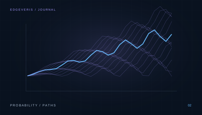
Win rate describes individual trades. Passing a challenge depends on an entire path. A strategy can win more than half its trades and still reach a loss boundary before its profit target. Monte Carlo analysis connects the trade distribution, position size, account rules and evaluation horizon. Its output is a conditional estimate, not a certificate of future success.
The practical objective is to answer a clear question: if the trading process behaved like the model, how often would it reach the target before a rule breach and before a specified deadline? A useful answer includes failures, unfinished attempts and uncertainty about the source data. Reporting only a smooth equity fan or one passing percentage leaves out most of the decision.
Start with a model simple enough to verify
Take an initial balance of $100,000, a target of $110,000 and a failure boundary of $90,000. Each completed trade adds or subtracts $1,000. The win probability is 55%, each outcome is independent, and the horizon is 100 trades. Stop at the first touch of either boundary. Deliberately omit daily limits, fees and open-position fluctuations in this teaching example.
Risk is fixed at 1% of the initial balance. It does not compound with current equity. After a loss, the next trade still risks $1,000. Changing that detail changes the reachable account values and the passing probability. A reproducible report should never describe both fixed-cash risk and current-equity risk simply as 1% without saying which basis is used.
| Outcome by trade 100 | Exact model probability | Meaning |
|---|---|---|
| Passed | 66.784% | Reached +$10,000 first |
| Failed | 8.978% | Reached −$10,000 first |
| Unfinished | 24.238% | Neither boundary reached |
These values can be calculated without random sampling. Keep the probability mass at every surviving integer profit state from −9 to +9. At each trade, move 55% of each state's mass one step upward and 45% one step downward. Absorb mass reaching +10 into passed and mass reaching −10 into failed. After 100 iterations, sum the remaining states to obtain unfinished probability.
This exact calculation is a valuable unit test for a Monte Carlo engine. A sufficiently large simulation of the same assumptions should approach these values within its sampling error. If it does not, check stopping order, boundary equality, compounding and whether failed paths accidentally continue trading.
Do not discard unfinished attempts
The three probabilities add to 100%. Among resolved attempts, the passing share is larger than 66.784%, but that is not the probability of passing within 100 trades. Removing unfinished attempts silently changes the question. Keep them visible, particularly when comparing conservative position sizes or strategies with few trading opportunities.
A chart of cumulative passing probability normally rises and then flattens as fewer live paths remain. The flattening can be legitimate. It can also reveal a horizon or scheduling bug. To distinguish the two, inspect the number of active paths at each step and verify that each path continues until its own terminal event or the actual horizon.
Time to pass should usually be summarized among passing paths and explicitly labeled that way. A median of 40 trades among successful attempts does not mean a typical purchased attempt will pass after 40 trades. Failed and unfinished attempts have different outcomes. A planning report should show their shares alongside conditional completion times.
Separate simulation error from uncertainty in the strategy
If the model's pass probability is around 67%, 10,000 independent simulated paths have a Monte Carlo standard error of roughly sqrt(0.67 × 0.33 / 10,000), or 0.47 percentage points. At 500,000 paths it falls to about 0.067 percentage points. More paths make the numerical estimate more stable, but they do not establish that the assumed 55% trading win rate is correct.
Suppose a historical sample contains 28 winning trades out of 50. Its observed win rate is 56%. A 95% Wilson interval for an independent binomial sample is approximately 42.3% to 68.8%. This interval describes uncertainty in a simplified constant-probability model. It is already wide before considering market changes, correlated trades, selection bias or errors in execution costs.
When those plausible win probabilities are fed into a boundary model, the range of pass probabilities can become much wider than the simulation's numerical error bars. That is why a result such as 66.8% should never be presented as a precise statement about a trader's real chance. The simulation is precise about its assumptions. The assumptions may be uncertain.
The Wilson interval is a frequentist procedure with a coverage interpretation across repeated samples. It is not literally a 95% probability that a fixed unknown win rate lies in this particular interval. For trading decisions, its practical value is to discourage treating a small historical sample as an exact parameter. NIST documents the calculation and its behavior for binomial proportions.
Use full trade outcomes when available
Real strategies rarely produce only +1R and −1R. They may have partial exits, small scratches, occasional large winners and losses exceeding the planned stop. Store each completed trade's net result divided by its planned entry risk. A $300 gain on a trade that initially risked $200 is +1.5R. A $260 loss on that same risk is −1.3R.
Sampling these observations with replacement preserves the empirical mixture of outcomes. One sampled path might contain the same historical trade several times and omit another. That is normal for a bootstrap. It differs from shuffling every observed trade exactly once, which holds the final total fixed and primarily explores ordering risk.
Check how transaction costs are included. If the source R values are already net of commissions and modeled slippage, do not subtract those costs again. If you stress an additional dollar of slippage, apply only the incremental cost with the correct number of contracts and sides. Otherwise an apparently conservative simulation can merely be double-counting expenses.
Preserve meaningful dependence
Independent trade resampling assumes that the sequence can be broken apart without losing important information. This is often unrealistic. Several trades may react to the same market event, or a strategy may lose throughout a low-volatility week. Resampling individual trades can distribute those losses more evenly than they occurred historically.
One alternative is to resample whole sessions. Another is a moving-block bootstrap that samples adjacent groups of observations. The block length expresses how much dependence you intend to preserve. Very short blocks can miss clustering, while very long blocks leave few effectively different samples. Compare several defensible lengths rather than optimizing the block size until the result looks attractive.
Daily-limit simulations especially need coherent sessions. Preserve the within-session trade order and, when available, intraday equity checkpoints. A daily loss boundary cannot be evaluated accurately from an unordered bag of daily closing balances. If a data set cannot establish open losses, describe the resulting limitation directly in the analysis.
Build a risk sensitivity curve
Repeat the same experiment across a modest grid of position sizes. Keep the random paths paired so differences are easier to interpret. For each size, report pass probability, failure probability, unfinished probability and time to pass. Do not select a size only because its base-case pass percentage is fractionally higher than its neighbors.
Look for a region that remains usable when costs rise or the estimated edge weakens. The historical best point can be a sampling accident. A small change from 0.9% to 1.0% risk may cause a discontinuity in a simple fixed-step model because a different number of losses reaches the boundary. That is a mathematical grid effect, not necessarily an economically meaningful optimum.
Position rounding matters too. A futures strategy cannot generally trade 0.37 standard contracts. Convert risk to allowable contract quantities and then recalculate the realized cash exposure. If the smallest trade exceeds the desired risk, the model should not invent fractional fills. A compatible smaller contract may help, but its fees and liquidity need their own assumptions.
Run adverse scenarios without pretending they are forecasts
A practical sensitivity table changes one assumption at a time. Increase average execution cost, reduce large winning outcomes, preserve longer loss clusters or evaluate a newer out-of-sample segment. These changes reveal which part of the estimated edge supports the passing probability. They are not predictions that a particular adverse scenario will occur.
Also test structural mistakes. Shift session boundaries to the correct timezone, include open losses, enforce minimum trading days and apply the actual trailing rule. These are not optional pessimistic scenarios if the contract requires them. They belong in the base model. Stress tests come after the contract itself is represented correctly.
If the strategy was chosen from hundreds of candidates, its observed trade sample is selected rather than neutral. Bootstrapping that winning sample alone does not correct the original selection process. Reserve untouched data, record how many alternatives were tried and avoid repeatedly choosing the version with the most flattering simulated pass rate.
A practical reporting checklist
- Name the code version and exact inputs behind the historical trades.
- State sample dates, trade count, costs and the definition of one R.
- Specify the program boundaries, timezone, risk basis and horizon.
- Identify whether paths use independent trades, sessions or blocks.
- Show passed, failed and unfinished proportions that sum to 100%.
- Report simulation precision separately from source-data uncertainty.
- Show sensitivity to weaker outcomes and realistic execution changes.
A useful conclusion might say that a selected setup performs acceptably under the base assumptions but becomes sensitive to clustered losing days. That observation tells you what to investigate. It is more actionable than claiming a universal 67% chance of passing. Monte Carlo is most useful when it exposes a dependency you can test, rather than concealing uncertainty behind a large number of simulated paths.